How to untangle neurons – What do large language models hide?

Developing large language models (LLM) is one of the biggest challenges in AI. What if, instead of passively analyzing their inner logic, we try to actively influence their actions? Here’s where sparse encoders come in handy, letting you tweak how the model behaves. But how can we do that?

Paulina Tomaszewska

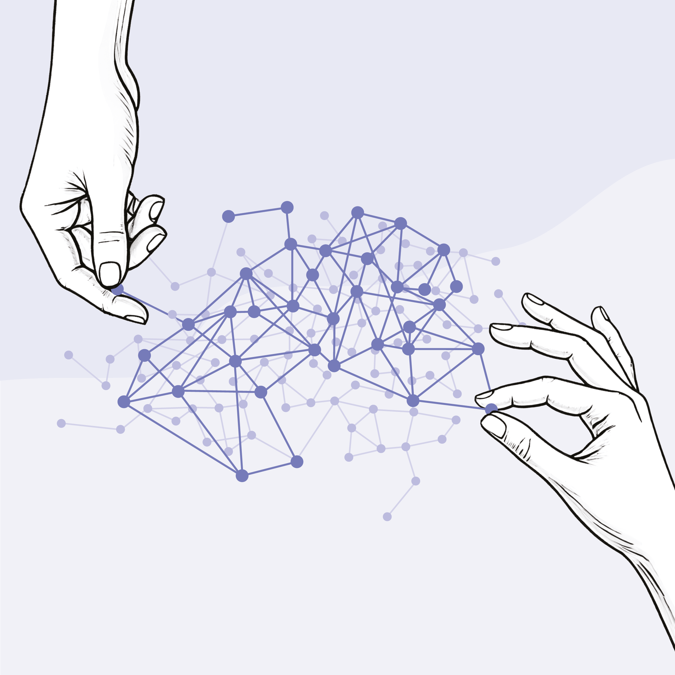
On the third issue of hAI Magazine, Michał Karpowicz explained the superposition hypothesis in neural networks. Basically, it assumes that neurons in such models are often polysemantic (ambiguous) – they don’t just represent one specific concept but many at the same time. Why is this happening? The number of concepts the model needs to “understand” during a task far exceeds the number of available neurons. As a result, neurons act as “multitasking” units, which makes interpreting them particularly difficult. Each neuron participates in processing many overlapping threads, creating a kind of “entangled network” of concepts and meanings.

Researchers have developed a method that lets us untangle these hidden neuron connections. For that purpose, they used sparse autoencoders (SAE). Interestingly, such models aren’t new – they appeared in the world of machine learning much earlier, but didn’t catch on back then. It was only recently, after they were used to analyze language models, that researchers got interested in them again. This is a great example of how old methods can make a comeback if they find a new, practical use.

What are sparse autoencoders?

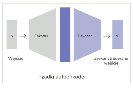
Autoencoders are most commonly associated with neural network pretraining techniques. Their basic role is to compress the input data in the encoder and then reproduce it by means of the decoder. In this process, it’s essential to keep all the important information in a compressed representation. To achieve this, classic autoencoders have a bottleneck between the encoder and decoder that forces a representation of data that’s minimal in terms of number of features, but rich in information.

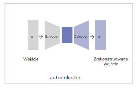
Sparse autoencoders work a bit differently, though. Unlike the classic ones, their hidden layer is larger than the input data size. In theory, this could lead to a situation where the model would just replicate the data 1:1, losing the ability to pick out important patterns. To prevent this, a sparsity requirement is introduced so that most values in the hidden representation are equal to zero. This way, sparse autoencoders can “untangle” individual concepts from the densely tangled web of dependencies in large language models, making them easier to interpret and control.

How does the training of a sparse autoencoder work?

The process starts by using a pre-trained large language model that operates in inference mode. The model extracts activations (internal data representations) from a selected layer. Then, these activations serve as input data for a sparse autoencoder (SAE). Most often, activation extraction takes place from the residual stream, which plays the role of a central memory resource in transformers. It’s right here that the results of the attention mechanism and dense layers are added, which allows information to flow efficiently between the model’s layers.

SAE training consists in minimizing reconstruction errors, as the model learns to map data as accurately as possible. At the same time, it applies regularization mechanisms that limit the number of active neurons in the hidden layer. As a result, only a small number of neurons activate for a specific input, making the autoencoder “sparse”.

Importantly, different sets of neurons activate in the SAE’s hidden layer for different sentences inputted into the language model. Thanks to the regularization applied, these neurons become selective – they only activate in response to specific concepts. This means that sparse autoencoders can effectively identify and separate the individual meanings that remain tangled in the activations of individual layers of large language models.

What can we “read” from SAE?

After finishing training a sparse autoencoder (SAE), you can inspect the hidden representations. It’s expected that the neurons in the hidden layer will be monosemantic – each should correspond to a single concept. The key challenge remains effectively identifying and labeling these neurons to figure out what concepts they represent.

The labeling process starts by making inferences on a trained SAE – for this purpose, a large text corpus is used. As a result of this operation, you can analyze which neurons in the hidden layer get activated in response to specific tokens. Then, you can assign labels to neurons by means of experts or using another large language model (that’s a way to automate the process). The annotation process with an LLM can include three stages:

Labeling – the LLM analyzes the tokens that triggered strong neuron activation and assigns a specific concept (label) based on that.
Activation prediction – assuming the assigned label is correct, LLM predicts the degree of neuron activation for the tokens that appear in the test sentences.
Comparison of results – the predicted activations from stage 2 are matched up with the actual activation values obtained from the original model by inference on the same test data. The measure of activation similarity determines how well the concept represented in the neuron was named.

If your goal is to analyze popular LLM architectures, you can often use pre-trained SAEs that are available online. The mapping of the meanings of individual neurons has been outlined on Neuronpedia.org – a kind of neuron atlas that makes it easier to interpret and explore their functions. For example, it includes information that in a given SAE, trained on activations from the residual stream in layer 6 of the GPT-2 Small model, the neuron with index 650 in the hidden layer was assigned the concept “length expressed in meters or feet”.

How to use SAE in practice?

Once you manage to untangle and name specific concepts in the hidden SAE layer, you can start to control a large language model so that, regardless of the received prompt, it refers to a specific chosen concept. The goal is to strengthen a particular concept in the model.

Anthropic researched have demonstrated that with this approach, you can make an LLM respond in a specific way – for instance, no matter what the question is about, the model could consistently refer to Golden Gate Bridge, for example.

Control is achieved by modifying activations (usually from the residual stream) in a selected layer L of a large language model LLM – the same one whose activations were used to train the SAE. Let’s label these activations as x_L. Here’s one of the most basic methods:

1. From Neuronpedia or through prior analysis, identify the neuron index i
in the hidden layer of the trained SAE that corresponds to the concept you’re interested in.
2. From the SAE decoder’s weights, take the vector corresponding to that neuron (control vector), V_decoder[i].
3. Modify the activations in the LLM, adding this control vector multiplied by some arbitrary constant: x_L : x_L + c * V_decoder[i].
4. Such transformed activations x_Lare reintroduced into the LLM model in the place from which they were originally extracted. Then, they flow through the next layers, influencing further processing stages and ultimately shaping the final response generated by the model.

If the constant c is properly chosen, the model will start giving answers that match what you expect. If the value is too high, the model will stop responding rationally and might start repeating the same token instead.

This approach opens up new possibilities in understanding and controlling the operation of large language models. We can intentionally reinforce or suppress specific concepts, adapting the model for various applications – from eliminating unwanted biases to forcing responses in a particular context and style.